Foreword
⁎ pretty basic, worth remembering
⁑ more detailed, not essential
⁂ nearly advanced, treat it as a fun fact
⁎ Machine Learning Model
A machine learning model is a statistical model (a function) that takes some representation of the data and returns predictions for this data. This function contains some trainable parameters.
We can denote input data representation as $x \in \mathcal{X}$ and the model as $f_\theta$, where $\theta$ is a set of model parameters. We will need an objective function $\mathcal{L}$ or a criterion to find the optimal set of model parameters for the given training data $\mathcal{D}$. Next, we define training as minimizing the objective with respect to the model parameters:
\begin{equation} \theta^* = {\arg\min}_{\theta} \,\, \mathcal{L}(f_\theta, \mathcal{D}), \end{equation}where $\theta^*$ is the optimal set of parameters for the given training dataset.
⁎ Supervised Learning
In supervised learning we will have a label $y \in \mathcal{Y}$ for each input data point $x \in \mathcal{X}$. Our training dataset will consist of such pairs $\mathcal{D} = \{ (x^{(i)}, y^{(i)})\}_{i=1}^N$.
In supervised learning we can have either discrete labels (classes), i.e. $y \in \{1, \dots, k\}$, or continuous labels $y \in \mathcal{Y} \subset \mathbb{R}$. The former problem is called ($k$-class) classification, and the latter is regression.
The objective function that we will be minimizing for regression is usually mean squared error: \begin{equation} \mathcal{L}(f_\theta, \mathcal{D}) = \frac{1}{N} \sum_{i=1}^N (f_\theta(x^{(i)}) - y^{(i)})^2 \end{equation}
⁎ Linear Regression
The linear regression model is one of the simplest machine learning models for the regression problem. In this case the input data point is represented as a vector $\mathbf{x}=[x_1, \dots, x_d]$ and the model parameters are also a vector $\boldsymbol\theta=[\theta_0,\dots,\theta_d]$. It is defined in the following way:
\begin{equation} f_\boldsymbol\theta(\mathbf{x}) = \theta_0 + x_1 \theta_1 + \dots + x_d \theta_d. \end{equation}The model prediction $\hat{y}$ is the value returned by this function ($\hat{y}=f_\boldsymbol\theta(\mathbf{x})$).
⁂ Optimization Problem
Let us use a simple regression example where the model input has only one feature $x$. The objective function then takes the following form:
\begin{equation} \mathcal{L}(f_\boldsymbol\theta, \mathcal{D}) = \frac{1}{N} \sum_{i=1}^N ( \underbrace{\theta_0 + x^{(i)}\theta_1}_{\hat{y}\,^{(i)}} - y^{(i)} )^2. \end{equation}It turns out that this function is convex, and we can minimize it analytically. Let us calculate the derivative w.r.t. the model parameters $\boldsymbol\theta$:
\begin{split} \frac{\partial\mathcal{L}(f_\boldsymbol\theta, \mathcal{D})}{\partial\theta_0} &= \frac{1}{N} \sum_{i=1}^N 2( \theta_0 + x^{(i)}\theta_1 - y^{(i)} ) = \\ &= \frac{2\theta_0}{N} \sum_{i=1}^N 1 + \frac{2\theta_1}{\color{red}N} \color{red}{\sum_{i=1}^N x^{(i)}} - \frac{2}{\color{orange}N} \color{orange}{\sum_{i=1}^N y^{(i)}} = 2(\theta_0 + \theta_1\color{red}{\bar{x}} - \color{orange}{\bar{y}}). \end{split}By setting this term equal to zero, we get the optimal solution: $\theta_0^* = \bar{y} - \theta_1\bar{x}$.
Doing the same for $\theta_1$:
\begin{split} \frac{\partial\mathcal{L}(f_\boldsymbol\theta, \mathcal{D})}{\partial\theta_1} &= \frac{1}{N} \sum_{i=1}^N 2x^{(i)}( \theta_0 + x^{(i)}\theta_1 - y^{(i)} ) = \\ &= \frac{2\theta_0}{N} \sum_{i=1}^N x^{(i)} + \frac{2\theta_1}{N} \sum_{i=1}^N \left(x^{(i)}\right)^2 - \frac{2}{N} \sum_{i=1}^N x^{(i)}y^{(i)} = \\ &= 2(\bar{y} - \theta_1\bar{x})\bar{x} + \frac{2\theta_1}{N} \sum_{i=1}^N \left(x^{(i)}\right)^2 - \frac{2}{N} \sum_{i=1}^N x^{(i)}y^{(i)}. \end{split}By substituting $\theta_0$ and setting this term equal to zero: \begin{split} 0 &= 2(\bar{y} - \theta_1\bar{x})\bar{x} + \frac{2\theta_1}{N} \sum_{i=1}^N \left(x^{(i)}\right)^2 - \frac{2}{N} \sum_{i=1}^N x^{(i)}y^{(i)} = \\ &= \theta_1\left(-2\bar{x}^2 + \frac{2}{N} \sum_{i=1}^N \left(x^{(i)}\right)^2\right) + 2\bar{x}\bar{y} - \frac{2}{N} \sum_{i=1}^N x^{(i)}y^{(i)} \\ &\implies \theta_1^* = \frac{\frac{1}{N} \sum_{i=1}^N x^{(i)}y^{(i)} - \bar{x}\bar{y}} {\frac{1}{N} \sum_{i=1}^N \left(x^{(i)}\right)^2 - \bar{x}^2}. \end{split}
⁎ Solution Applied
Now, we can apply the derived solution by calculating $\theta_1^*$ and substituting it to $\theta_0^*$.
⁎ Model Evaluation
We now can clearly see that our model can be fit to the data, but how can we evaluate its performance for the future use cases?
Typically, the dataset is split into two subsets: training and testing sets. The testing set can be for example 20% of compounds that were not used in training, and are held-out for the final evaluation using evaluation metrics. These metrics can be different depending on the solved task, e.g. regression and classification tasks will have different metrics.

⁎ Time-Based Split
The random split in which random X% instances are moved to the training set is commonly used in many application, but in chemistry can lead to wrong assumptions. We would like to split data in a way that accurately evaluates the model performance on prospective tasks and its generalization to out-of-distribution data. One of the propositions could be splitting by time, which simulates how models are used in practice: we take all the data we have for training and then use it for the compounds synthesized in the future.

⁎ Scaffold-Based Split
Scaffold-based split is another criterion that can be used to split compounds to test the generalization of the ML algorithm. In this approach, all the compounds are assigned to bins based on the substructures called Bemis-Murcko scaffolds, which are core substructures after removing all side chains. Next, these bins are assigned to different training/testing sets to minimize the similarity of compounds between these sets.
This split can be implemented in several different ways, e.g. it can create bins based on only 3-ring systems included in the BM scaffold, or only generic scaffolds with atom and bond identities removed are used. One of the disadvantages of this splitting method is that all acyclic compounds are assigned to the same set (their scaffold is "empty").

⁑ Clustering-Based Split
Another option for splitting compounds according to their similarity is a clustering-based split. In this method, compound fingerprints (usually ECFP) are computed, and the data is clustered using the Taylor-Butina clustering method (also known as the sphere exclusion clustering) with the distance threshold $t$ as the only parameter:
- The set of clusters is initialized as an empty set.
- A random unprocessed compound $c$ is sampled;
- if the Tanimoto similarity between $c$ and the closest cluster is less than $t$, assign $c$ to this cluster.
- Otherwise, create a new cluster with $c$ as its center.
- Repeat step 2 until all compounds are assigned.
⁎ Metrics
For evaluating machine learning models, some evaluation metrics need to be selected to compare model results on the testing data. Depending on the task, we can calculate regression or classification metrics. During this lecture, we will focus on the regression problem and binary classification, as those are the most common tasks in molecular property prediction.
Regression Metrics
In regression, we usually calculate an average error of the model. Two metrics that we use are Mean Absolute Error (MAE) or Root Mean Squared Error (RMSE). Sometimes we are more concerned about the correlation between predictions and the data, and the explained variance, in which case we can use the R$^2$ coefficient.
\begin{equation} \text{MAE}(\mathbf{y}, \mathbf{\hat{y}}) = \frac{1}{N} \sum_{i=1}^N |y_i - \hat{y}_i| \end{equation}\begin{equation} \text{RMSE}(\mathbf{y}, \mathbf{\hat{y}}) = \sqrt{\frac{1}{N} \sum_{i=1}^N (y_i - \hat{y}_i)^2} \end{equation}\begin{equation} \text{R}^2(\mathbf{y}, \mathbf{\hat{y}}) = 1 - \frac{\sum_{i=1}^N (y_i - \hat{y}_i)^2}{\sum_{i=1}^N (y_i - \bar{y})^2},\quad \bar{y} = \frac{1}{N}\sum_{i=1}^N y_i \end{equation}Binary Classification Metrics
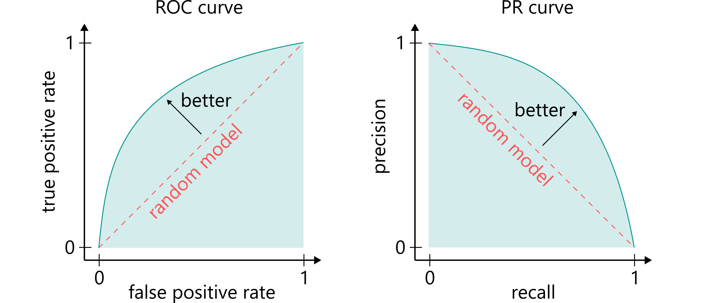
The simplest evaluation metric for classification is accuracy, which is the number of correctly predicted compounds divided by the total number of tested compounds. However, this metric does not work well when the number of compounds in the positive class is much smaller (or greater) than in the negative class. Thus, we often use ROC AUC or PR AUC in these cases. These metrics calculate the area under the receiver operating characteristic curve or under the precision-recall curve.
⁎ Hyperparameter Search
Most of the ML algorithms can take additional non-trainable parameters (hyperparameters) that impact the model performance. For example, the random forest algorithm can take the maximum height of decision trees or the number of trees in the forest. To find the optimal set of hyperparameters, we can use a validation set. It is important not to tune the hyperparameters using the testing set as it may make the calculated metrics too optimistic (the hyperparameters are tuned using the testing set, so this set is visible in the training process).
We can create a validation set in a similar way to the testing set, e.g. the dataset can be split into 70% of the training compounds, 10% of the validation compounds, and 20% of the testing compounds.
Pseudocode:
for hyperparams in hyperparameter_grid:
    model = train(hyperparams, training_data)
    valid_metric = score(model, validation_data)
    best_model = update_best_model(model, valid_metric)
test_metric = score(best_model, testing_data)
⁑ Cross-Validation
A more strict method of hyperparameters tuning is cross-validation. In this procedure, the dataset is split into $k$ folds, and the calculations are repeated $k$ times, each time using the $k$-th fold as the validation set. The best hyperparameters are chosed based on the best average metric value for all folds.

Pseudocode:
for hyperparams in hyperparameter_grid:
    valid_metric = 0
    for training_folds, validation_fold in folds:
        model = train(hyperparams, training_folds)
        valid_metric += score(model, validation_fold)
    best_model = update_best_model(model, valid_metric / n_folds)
test_metric = score(best_model, testing_data)
⁎ Neural Networks
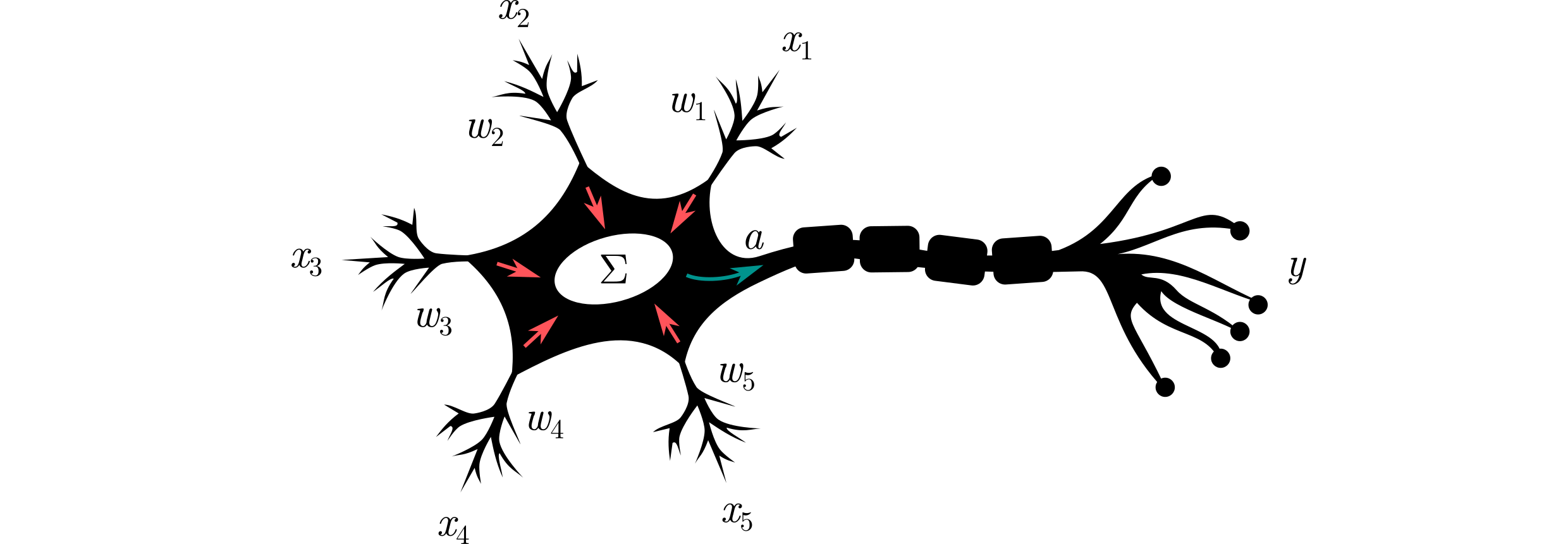
Artificial neural networks (ANNs) are ML models that are inspired by the way biological neurons work. In a nutshell, a neuron collects (electrochemical) signals from other neurons and fires when it is stimulated to a certain level. This can be described by the equation:
\begin{equation} f_\mathbf{w}(\mathbf{x}) = a(w_1x_1 + w_2x_2 + \dots + w_dx_d), \end{equation}where $\mathbf{x}$ is the input vector (or signals from the other neurons), $\mathbf{w}$ are the connection weights (model parameters), and $a:\mathbb{R}\to \{0,1\}$ is the step activation function. Can you see an analogy to the linear regression model?
⁎ Multi-Layer Networks
In ANNs, neurons are arranged in layers that are processed sequentially. Each layer computes another level of abstraction of the input data. The network input is the vector representation of the data. After passing through a neural layer, the data is transformed into a so-called hidden representation, which is computed combination of the input features. This operation can be repeated a few times before the network output is returned after the last layer.

⁎ Computations
Let us denote the layer input as $X\in\mathbb{R}^{N\times h_{\text{in}}}$. A forward pass thorugh a fully-connected layer with weights $W\in\mathbb{R}^{h_{\text{in}}\times h_{\text{out}}}$ can be computed in the following way:
\begin{equation} H = XW \in \mathbb{R}^{N\times h_{\text{out}}} \end{equation}Let us assume that our input data consists of $N$ compounds encoded as $d$ features (e.g. a fingerprint of length $d$). The input data can be then represented as a design matrix $X\in\mathbb{R}^{N\times d}$, where $i$-th row ($\mathbf{x}_i$) is the encoding of the $i$-th compound. The trainable parameters (called weights) in $l$-th layer are denoted $W^{(l)}$. The forward pass (prediction) is computed as:
\begin{equation} \mathbf{\hat{y}} = \sigma\left(XW^{(1)}\right)W^{(2)}, \end{equation}where $\sigma$ is an activation function, $W^{(1)}\in\mathbb{R}^{d\times h}$, $W^{(2)}\in\mathbb{R}^{h\times 1}$. Why do we need an activation function here?
⁎ Activation Functions
Activation functions are non-linear functions that allow neural networks to learn non-linear relationships between data features and labels. Without activations, deep neural networks cannot learn anything more than a linear regression model. Consider the following example of 2-layer network without activations:
\begin{equation} \mathbf{\hat{y}} = \left(XW^{(1)}\right)W^{(2)} = X\left(W^{(1)}W^{(2)}\right) = X\tilde{W}. \end{equation}We can see that this whole network can be translated to a one-layer model with weights $\tilde{W}$ equal to the multiplication of all layers weights (linear regression).
⁎ Training
The optimal solution of neural networks training can be difficult to find analytically. Networks can have different numbers of layers and activation functions. This makes the optimization problem intractable. What is more, the MSE objective function is not convex w.r.t. the network weights. Let us go back to the same problem as discussed for the linear regression model, but let us use the 2-layer network defined above.
⁎ Gradient Descent
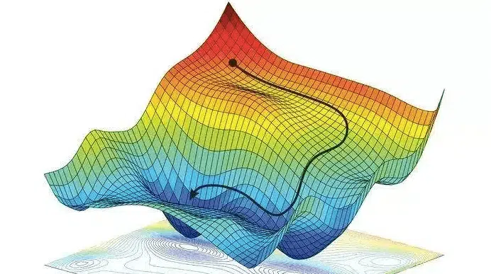
The optimization of deep neural networks is nontrivial, so iterative methods using gradients are used. In the first step, the forward pass is calculated to get the model predictions. Next, the loss function value is calculated, and an automatic differentiation method is employed to calculate gradients w.r.t. all the model trainable weights. These gradients are used to modify weights to get closer to the optimal solution, e.g. using the stochastic gradient descent (SGD) formula below. The process is repeated until convergence.
\begin{equation} W \leftarrow W - \eta \nabla_W\mathcal{L}, \end{equation}where $\eta$ is the learning rate (the step size in each iteration), and $\nabla_W\mathcal{L}$ is the loss function gradient w.r.t. the model weights $W$. The term "stochastic" is used because in each step we typically use a random sample of the training set, called a batch.
⁑ GPU Support
When training neural networks, we can take advantage of GPUs which accelerate computation. GPUs have higher memory bandwidth and can use parallelization to calculate multiple outputs at the same time. This is particularly useful in matrix multiplication, where all elements of the output matrix can be calculated independently. Matrix multiplication is the most often used operation in neural networks. Additionally, GPUs have fast access memory that can be used to store data. One of the reasons we need to use batches to train neural networks is that sometimes we cannot fit all the data into memory (but there are other, even more important, reasons from the optimization standpoint).
$$ \begin{bmatrix} a_{11} & a_{12} & \cdots & a_{1n}\\ a_{21} & a_{22} & \cdots & a_{2n}\\ \vdots & \vdots & \ddots & \vdots\\ a_{m1} & a_{m2} & \cdots & a_{mn} \end{bmatrix} \times \begin{bmatrix} b_{11} & b_{12} & \cdots & b_{1p}\\ b_{21} & b_{22} & \cdots & b_{2p}\\ \vdots & \vdots & \ddots & \vdots\\ b_{n1} & b_{n2} & \cdots & b_{np} \end{bmatrix} = \begin{bmatrix} c_{11} & c_{12} & \cdots & c_{1p}\\ c_{21} & c_{22} & \cdots & c_{2p}\\ \vdots & \vdots & \ddots & \vdots\\ c_{m1} & c_{m2} & \cdots & c_{mp} \end{bmatrix} $$ $$ c_{ij}= a_{i1} b_{1j} + a_{i2} b_{2j} +\cdots+ a_{in} + b_{nj} = \sum_{k=1}^n a_{ik}b_{kj} $$
⁎ Classification
To adapt our neural network to the classification problem, we need to change a few elements of the architecture. First, we need to make sure that our output represents the predicted class. For binary classification we can use the sigmoid activation at the end, which takes values in the range from 0 to 1. If the predicted value is below 0.5, we can assume that the predicted class is 0, and 1 otherwise. To train such a network, we can use the binary cross-entropy loss function:
\begin{equation} \text{BCE}(\mathbf{y}, \mathbf{\hat{y}}) = -\frac{1}{N} \sum_{i=1}^N y_i \log \hat{y}_i + (1-y_i) \log (1-\hat{y}_i) \end{equation}⁎ Graph Neural Networks
Up to this point, we needed to convert molecules to vector representations in order to use them for ML model training. Although these representations work well in many scenarios, they are not a natural representation of chemical compounds, but rather sets of handcrafted features or structural motifs. A more natural representation for molecules are molecular graphs which correspond to the structural formulas of these compounds. To process this type of information, graph neural networks were designed, which can work directly on molecular graphs.
⁎ Molecular Graphs
Molecular graphs are attributed graphs in which vertices represent atoms and edges represent chemical bonds. The graph is attributed because each vertex (oftentimes also each bond) is attributed with some features that makes it possible to identify atom types (element symbol) and bond orders. These graphs are undirected.
Formally, we can define a molecule as an attributed graph $\mathcal{G}=(V,E,a_V,a_E)$, where $V$ is the set of vertices (atoms), $E$ is the set of edges (bonds), and $a_V$, $a_E$ are functions that map vertices and bonds to their features.
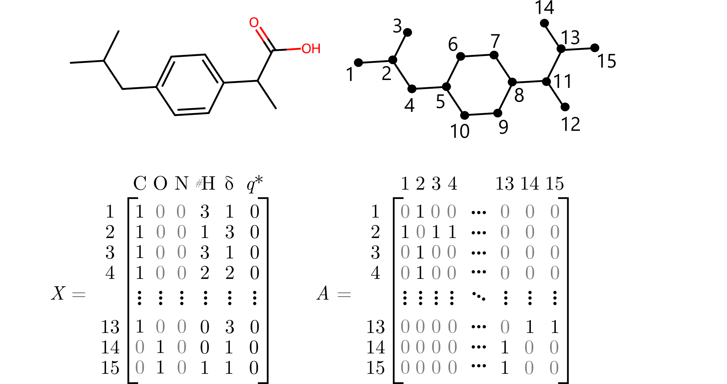
Graphs can be represented using the matrix representation, where $X\in\mathbb{R}^{n\times d}$ is the matrix of atomic features, and $A\in\{0,1\}^{n\times n}$ is the adjacency matrix. The $i$-th row of $X$, $\mathbf{x}_i$, is a feature vector corresponding to the $i$-th vertex. The element $a_{ij}$ of the matrix $A$ is equal 1 if and only if there is an edge between the $i$-th and $j$-th vertex. We can also use a bond features tensor $B\in\mathbb{R}^{n\times n \times b}$ to represent edge features.
Example
Molecular features can include one-hot encoded atom types (C, O, N), number of implicit hydrogens (#H), number of heavy neighbors ($\delta$), or formal charge ($q^*$).
⁎ MPNN
Message passing (MP) is currently one of the most widely used frameworks for graph neural networks. In this framework, information is carried throughout the graph by edges that transfer messages. The edge message from the $i$-th vertex to the $j$-th vertex is defined as:
\begin{equation} \mathbf{m}_{ij} = M(\mathbf{x}_i, \mathbf{x}_j, \mathbf{b}_{ij}). \end{equation}Next, the vertex message is calculated by aggregating all incoming messages:
\begin{equation} \mathbf{m}_i = \sum_{j\in\mathcal{N}(i)} \mathbf{m}_{ji}, \end{equation}where $\mathcal{N}(i)$ is the neighborhood of the $i$-th vertex (a set of all directly connected vertices). Finally, the vertex representation is updated: \begin{equation} \mathbf{x}_i \leftarrow U(\mathbf{x}_i, \mathbf{m}_i). \end{equation}
Note that this is a general framework, and the funtions $M$ and $U$ can be chosen arbitrarily.
The message passing operation can be repeated multiple times before the vertex messages are aggregated as one vector representation for the whole molecular graph: \begin{equation} \mathbf{g} = R(X), \quad \text{where $R$ can be chosen arbitrarily, e.g. } R(X) = \frac{1}{n} \sum_{i=1}^n \mathbf{x}_i \end{equation}

⁎ GCNs
Now, we will look at a concrete example of a message passing neural network. Graph convolutional networks (GCNs) are a simple example of a graph neural network, in which messages from the neighboring vertices are collected by multiplying node vectors by weights (trainable model parameters) and normalizing them by the node degrees.
\begin{equation} \mathbf{m}_{ij} = \frac{1}{\sqrt{\delta_i\delta{j}}} W\mathbf{x}_i, \quad \mathbf{x}_i \leftarrow \sum_{j\in\mathcal{N}(i)} \mathbf{m}_{ji}. \end{equation}We can also use matrix notation to update all nodes in one step. Usually we assume that self-loops are added to the graph, i.e. $\hat{A} = A+I$, and we denote the diagonal degree matrix as $\hat{D}_{ii}=\sum_{j=1}^n \hat{A}_{ij}$. The GCN layer can be then calculated as: \begin{equation} X \leftarrow \hat{D}^{-1/2}\hat{A}\hat{D}^{-1/2}XW^T \end{equation}
⁑ GIN
In graph-based prediction tasks, it is important that graph neural networks are able to tell apart different graphs. However, this is quite a challenging as the graph isomorphism problem may be NP-intermediate. It was shown that current graph neural networks have at least the same power as the Weisfeiler-Lehman test for graph isomorphism. This topic was first raised in the paper that proposed a new architecture, graph isomorphism network (GIN), that addresses this problem. The GIN layer can be defined in the following way: \begin{equation} \mathbf{x}_i \leftarrow h_\boldsymbol\theta\left((1+\epsilon)\cdot\mathbf{x}_i + \sum_{j\in\mathcal{N}(i)} \mathbf{x}_j \right), \end{equation} where $h_\boldsymbol\theta$ is a neural network, and $\epsilon$ is a hyperparameter.
⁂ GAT
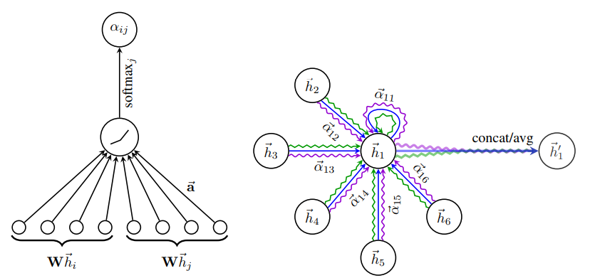
The architectures described above are powerful, but they share one issue (or feature?). All neighboring nodes are aggregated using the same weights because in graphs we do not have any particular ordering of nodes (these methods are also invariant to node permutation). Graph attention network (GAT) is a solution for this problem that uses attention to tell apart different node neighbors. The GAT layer is defined as: \begin{gather} \mathbf{x}_i \leftarrow \alpha_{ii}W\mathbf{x}_i + \sum_{j\in\mathcal{N}(i)} \alpha_{ij}W\mathbf{x}_j,\\ \alpha_{ij} = \frac{\exp\left( \text{LeakyReLU}(\mathbf{a}^T [W\mathbf{x}_i\|W\mathbf{x}_j] \right)}{\sum_{k\in\mathcal{N}(i)} \exp\left( \text{LeakyReLU}(\mathbf{a}^T [W\mathbf{x}_i\|W\mathbf{x}_k] \right)}, \end{gather} where $\|$ is the concatenation operator, and $\mathbf{a}$ is a trainable parameter.
⁂ MAT
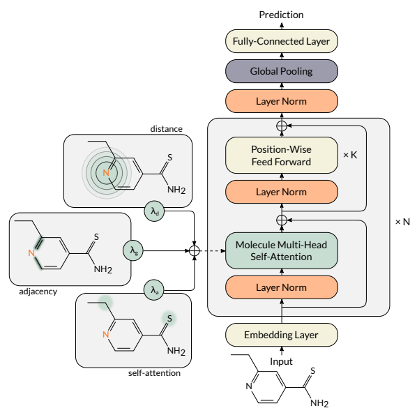
All the architectures above use local information (neighborhood) to update node representations. However, sometimes longer-range dependencies may become useful in molecular property prediction tasks. To tackle this issue, several graph transformers were proposed, in which longer-range dependencies are modeled by the self-attention mechanism. One example of a molecular graph transformer is Molecule Attention Transformer (MAT). Its multi-head molecule self-attention layers combine three sources of information: local graph topology, global self-attention, and inter-atomic distances. This operation is defined as: \begin{equation} X \leftarrow \Big\|_{i=1}^H \left( \lambda_a \rho\left(\frac{Q_iK_i^T}{\sqrt{d_k}}\right) + \lambda_d g(D) + \lambda_g A \right)V_i, \end{equation} where $H$ is the number of self-attention heads, and $\lambda_a$, $\lambda_d$, and $\lambda_g$ are hyperparameters. Let us split this equation into parts.
The selected fragment corresponds to a simple unnormalized graph convolution, $V_i=XW_i^V$ is a part of the self-attention mechanism, but is calculated almost exactly as in GCN. \begin{equation} X \leftarrow \Big\|_{i=1}^H \left( \lambda_a \rho\left(\frac{Q_iK_i^T}{\sqrt{d_k}}\right) + \lambda_d \color{red}{g(D)} + \lambda_g A \right)\color{red}{V_i}. \end{equation} This part is a similar operation as graph convolution, but uses continuous values (inter-atomic distances) instead of the binary adjacency matrix. The function $g$ can be an arbitrary transformation of distances, but we usually use $g(d)=e^{-d}$ so that the importance of the further atoms decreases exponentially. \begin{equation} X \leftarrow \Big\|_{i=1}^H \left( \lambda_a \color{red}{\rho\left(\frac{Q_iK_i^T}{\sqrt{d_k}}\right)} + \lambda_d g(D) + \lambda_g A \right)\color{red}{V_i}. \end{equation} Finally this is the classical self-attention, where $\rho$ is the softmax function, $d_k$ is the vector dimension, and $Q_i=XW^Q_i$, $K_i=XW^K_i$, and $V_i=XW^V_i$ are queries, keys, and values of the self-attention mechanism.
⁎ 3D Molecular Graphs
For many applications in drug discovery, it is beneficial to consider not only the structural (topological) graph information, but also molecular conformations. Let us extend our definition of a molecular graph by adding positions $R\in\mathbb{R}^{n\times 3}$, where $\mathbf{r}_i$ corresponds to the position of the $i$-th atom in the 3-dimensional Euclidean space.
You appear to be running in JupyterLab (or JavaScript failed to load for some other reason). You need to install the 3dmol extension:
jupyter labextension install jupyterlab_3dmol
⁑ SGCN
Spatial graph convolutional network (SGCN) is an example of a graph neural network that can effectively use spatial atom positions. The spatial graph convolution assigns different weights for each of the atom neighbors based on their relative positions. This operation is defined in the following way:
\begin{equation}
\mathbf{x}_i \leftarrow h_\boldsymbol\theta \left( \Big\|_{k=1}^K \sum_{j\in\mathcal{N}(i)} \text{ReLU}(W_k^T(\mathbf{r}_j-\mathbf{r}_i)+\mathbf{b}_k) \odot \mathbf{x}_j \right),
\end{equation}
where $K$ is the number of convolutional filters, $W_k$ and $\mathbf{b}_k$ are trainable parameters, and $\odot$ is the Hadamard multiplication (element-wise multiplication).

⁎ E(3)-Equivariance
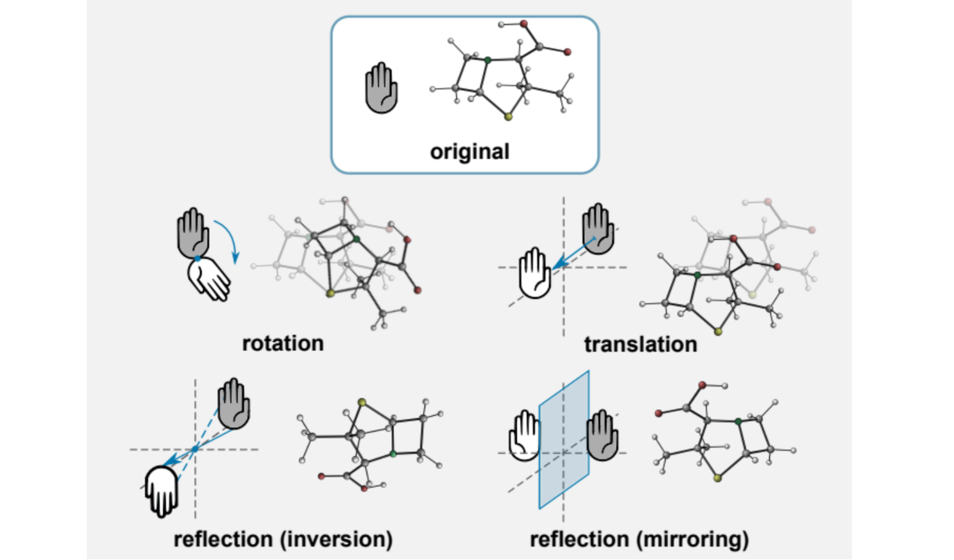
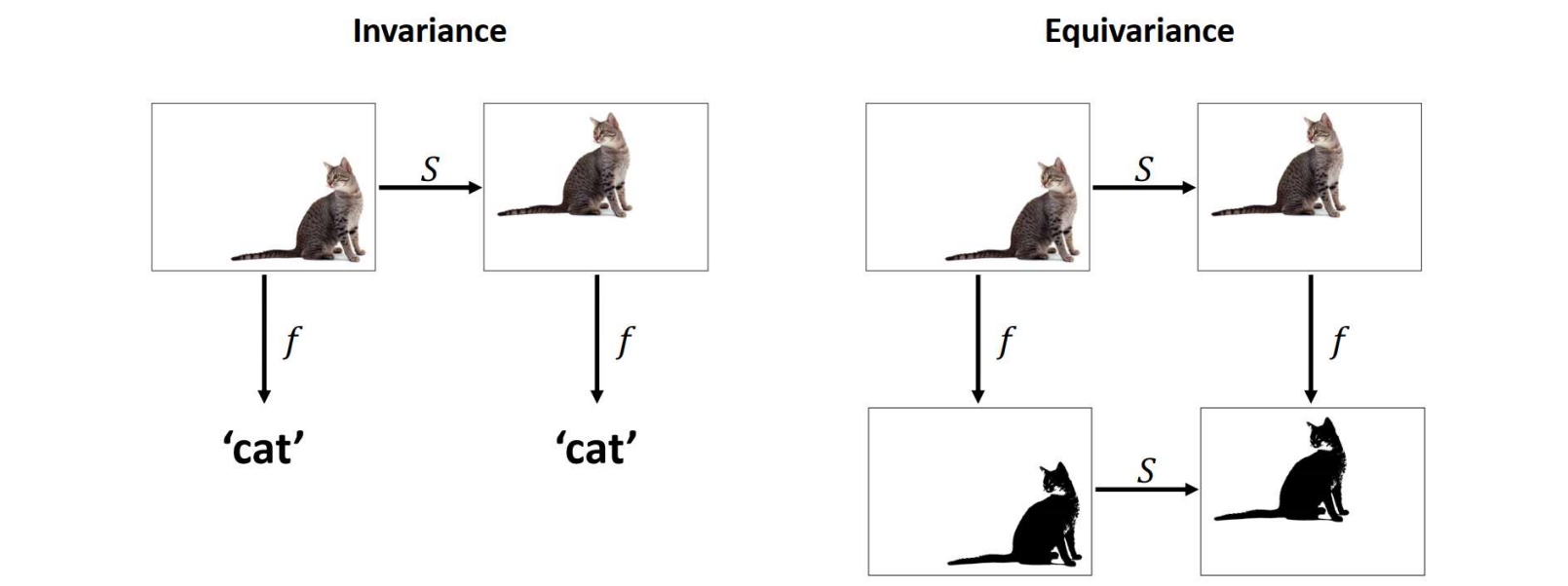
SGCN can use spatial positions but is only invariant to translations, and not invariant to rotations. To achieve rotational invariance, the conformations need to be randomly rotated during training (using random data transformations is called data augmentation). However, some neural network architectures are designed to be invariant (or equivariant) to some transformation groups, e.g. Euclidean group E(3) that preserves Euclidean distances.
źródło: https://www.doc.ic.ac.uk/~bkainz/teaching/DL/notes/equivariance.pdf
⁂ SchNet
SchNet is one of the E(3)-invariant architectures. It uses interatomic distances to construct weights. Because distances are invariant to rotations and translations (but also to reflections), we get an E(3)-invariant architecture. The SchNet continuous-filter convolution is defined as: \begin{equation} \mathbf{x}_i \leftarrow \sum_{j\in V} \mathbf{x}_j \odot W(\mathbf{r}_i - \mathbf{r}_j), \end{equation} where $W$ is a filter-generating function that can be defined as: \begin{equation} W(\mathbf{r}_i - \mathbf{r}_j) = h_\boldsymbol\theta\left( \Big\|_{k=1}^K e_k( \mathbf{r}_i - \mathbf{r}_j ) \right) = h_\boldsymbol\theta\left( \Big\|_{k=1}^K \exp\left( -\gamma \| d_{ij} - \mu_k \|^2 \right)\right), \end{equation} where $\gamma=10$ and $\mu_k\in\{0, 0.1, 0.2, \dots, 30 \}$ are hyperparameters, $d_{ij} = \| \mathbf{r}_i - \mathbf{r}_j \|$.
⁎ Protein Representations
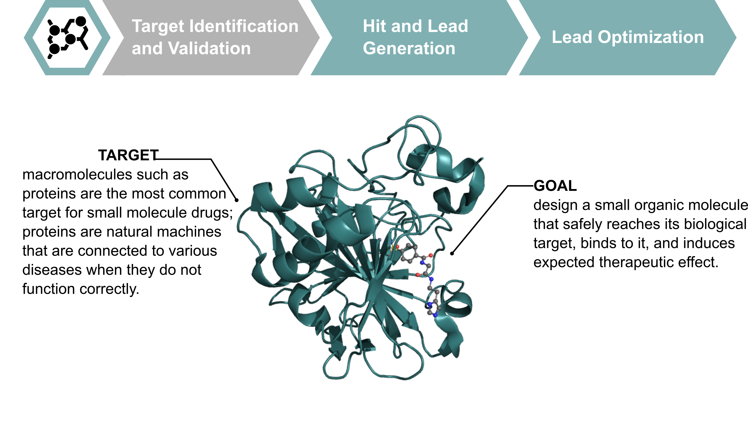
Proteins are macromolecules that are often considered as drug targets. The goal of the design of a therapeutic compound can be to activate or inhibit one of the proteins. For the visualization purposes, proteins are often depicted using the cartoon representation that shows the protein secondary structure (mostly $\alpha$-helices and $\beta$-structures). Below you can see a small molecule (ligand) inside a binding pocket of the protein.
⁎ Graph Representation
Proteins, as other molecules, can be represented as molecular graphs. However, this is not the most efficient representation in this case. Proteins are polymers (sequences) of amino acids. Only 20 amino acids are commonly found in proteins, so the polymer chains are combinations of these substrucutres repeated in a specific order.
⁎ Backbone Graph
To remove redundancy from the protein graph, sometimes only protein backbone is encoded. In this representation, $\alpha$-carbons in the backbone chain are nodes, and its encoding contains information about which amino acid is attached to this carbon. These carbons can be connected by edges to create a graph, or they can be processed as point clouds.
⁎ Voxel Representation
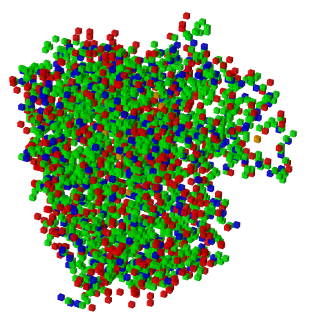
In voxel representation, a 3D grid of voxels (cubes) is defined around the protein. If an atom falls inside one of the voxels, its encoding (atom type) is encoded in this voxel. This representation is similar to image data but has one more dimension (images are 2D grids of pixels). Thus, voxelized proteins can be processed using 3D convolutional neural networks.
⁎ Binding Site Prediction
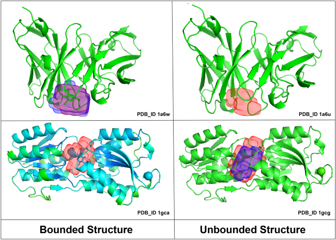
Protein representations can be used for binding site/pocket prediction, which conceptually is similar to image segmentation.
⁎ Binding Prediction
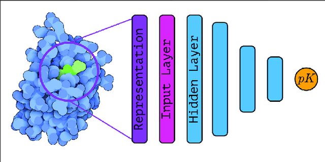
Binding affinity can be predicted by combining ligand and protein representations.
⁎ Generative Models
Generative models are used to create new instances that are similar to the examples in the training set. Generative models in drug discovery are also known as inverse molecular design because typically additional property- or structure-related goals are imposed. In unconstrained generation, we can measure compound validity, novelty, and uniqueness. In property- or structure-constrained molecular generation, we also check the optimization constraints, e.g. predicted properties.
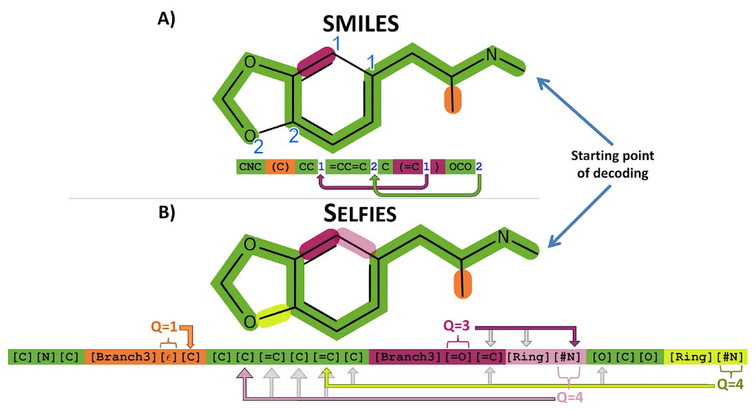
Molecules can be generated using 1D, 2D, or 3D representations. 1D representations are textual representations, 2D representations are structural/graphical representations, and 3D representations are 3D graphs and point clouds.
⁎ 1D Representations
⁎ Architectures
Deep generative models are neural networks that have their outputs adapted to generating molecular representations. There are several training schemas known from other fields, like natual language processing or computer vision, that were employed to compound generation.
⁎ Autoencoders
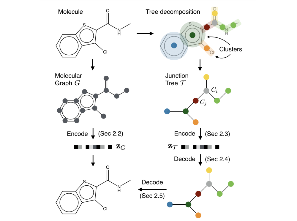
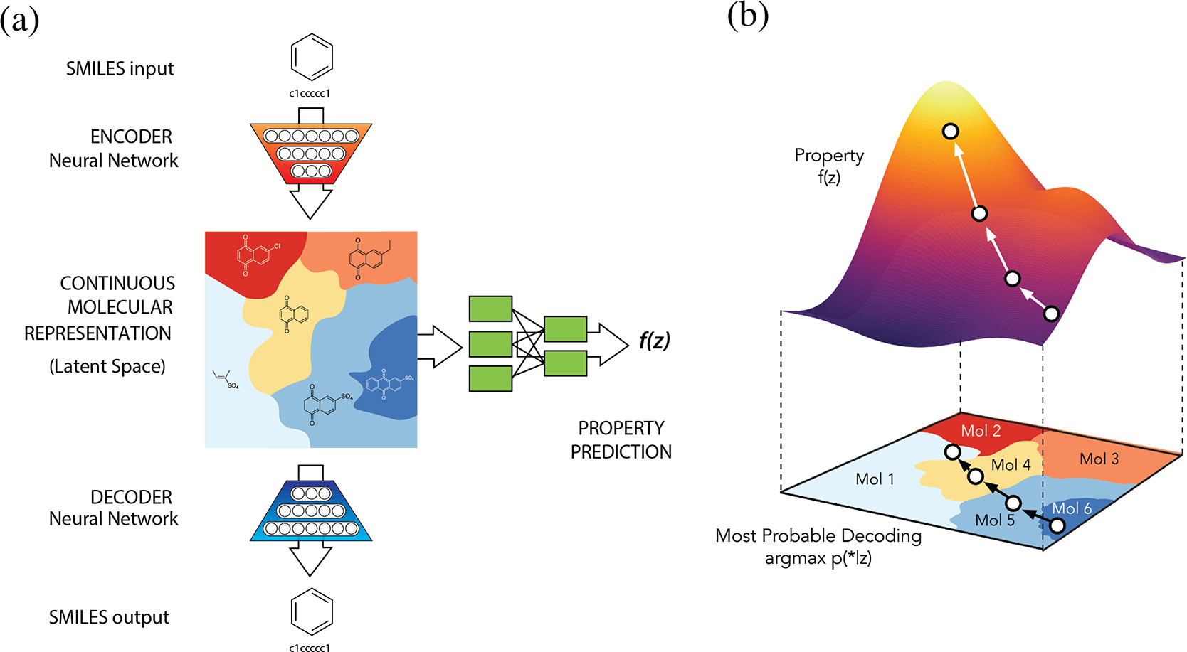
Autoencoders are models that consist of two neural networks: encoder, that encodes the input molecule into a low-dimensional latent space, and decoder, that decodes the latent space representation back to the molecule space. The loss function of this model has two components: (1) the reconstruction loss, that minimizes the distance between the input and reconstructed molecules, and (2) latent space regularization, that maximizes the similarity between the latent space distribution and some known distribution (usually the Gaussian distribution). In variational autoencoders (VAE), the second term is the Kullback-Leibler divergence between the latent space and the Gaussian distribution.

⁎ GANs
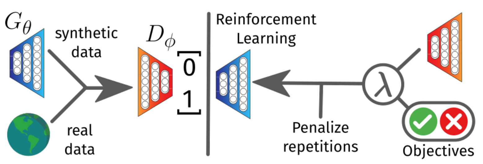
Generative adversarial networks (GANs) are a less popular choice than VAE in cheminformatics. This model also consists of two networks: a generator, that generates new molecules from a random Gaussian noise, and a discriminator, that learns to distinguish between real molecules and the generated ones. The training process is a min-max game in which the generator tries to deceive the discriminator, which in turn gets better and better at detecting fakes.
GANs are not commonly used in drug discovery because they need to propagate gradients through the generated discrete molecules in order to learn.

⁎ Flow Models
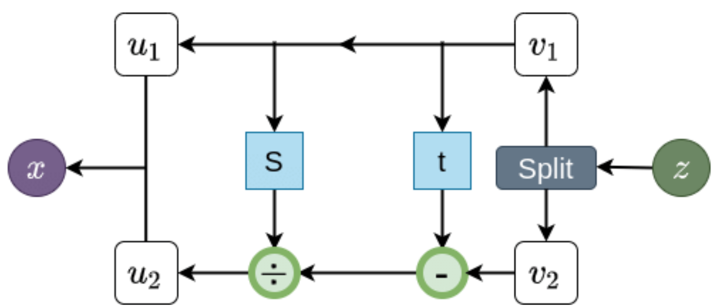
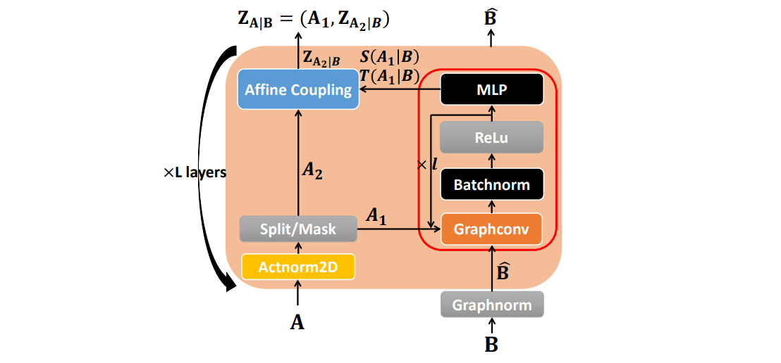
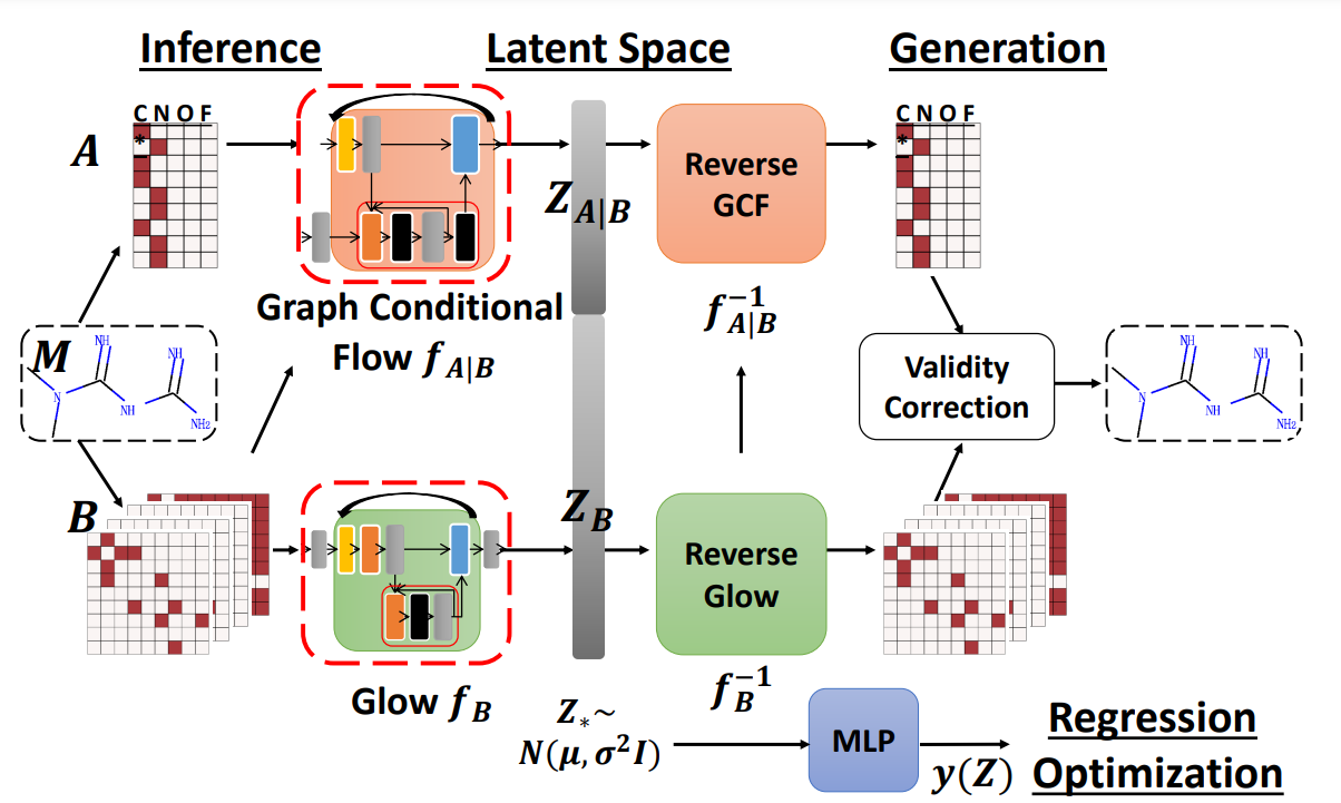
Normalizing flow models are neural networks composed only of invertible layers. They are trained to map the input distribution to the Gaussian distribution, and then they can be used to generate new molecules by sampling from the Gaussian noise. Flows can also be used to estimate likelihood of the data. The disadvantage of flows is that their layers need to satisfy certain conditions which may hurt the transformation flexibility.

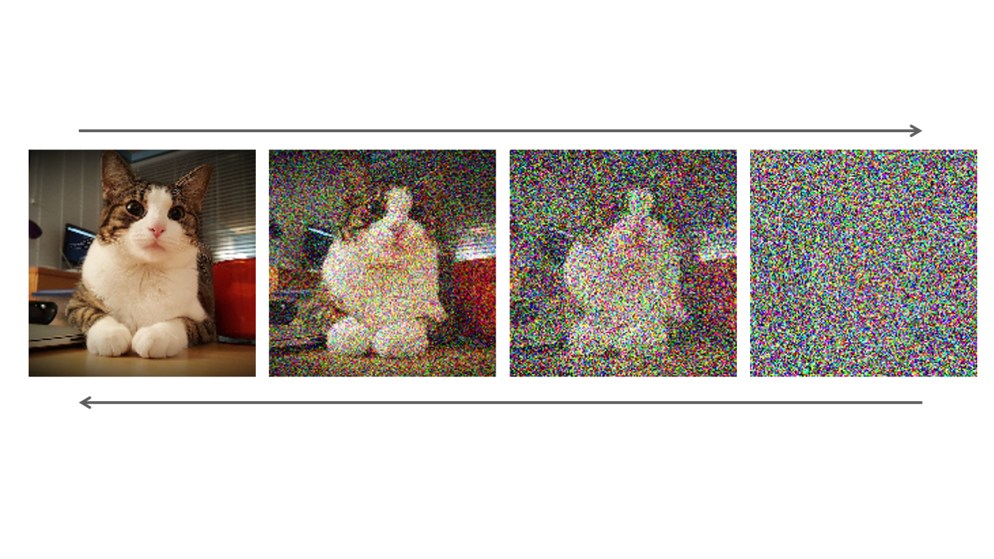
⁎ Diffusion Models
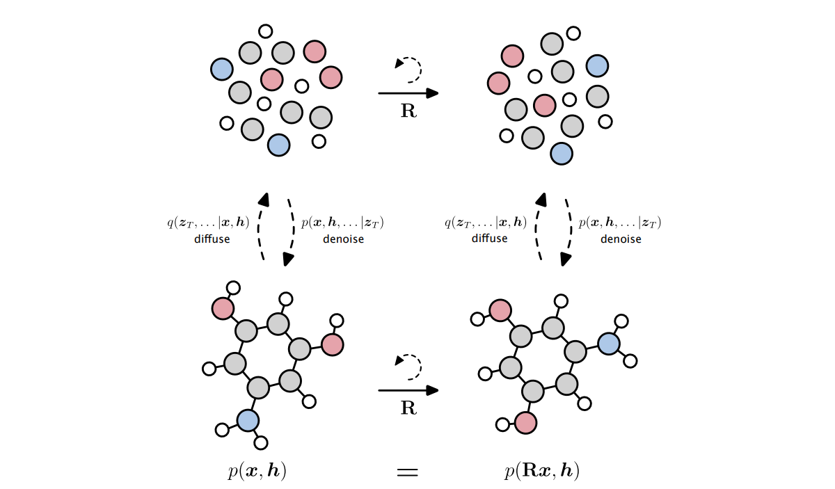
Diffusion models are two-stage models. In the first stage, the forward diffusion process, the input data is gradually perturbed by adding Gaussian noise. The second stage, the reverse diffusion, the model learns how to denoise the data to get the initial sample.
